Prodigy optimizer

Learning Rate (LR) tuning is very tedious for neural networks. Methods like $\mu$P [5] can help alleviate pain by enabling hyperparameter transfer from small to large models, but an LR sweep is still necessary. There is some work on the eradication of the LR sweep [1,2,3,4,6], with Prodigy being one promising solution (see here).

Here, we aim to understand how Prodigy works. When seeing the Algorithm for the first time, it's completely non-obvious what it's trying to do. We see that it's tracking several EMAs, and taking some sort of Adam-like descent step (line 11), but the motivation is unclear. Amazingly we can understand it by considering optimization of a convex function with gradient descent, which is what we do here.

We also run a quick experiment to compare versus AdamW.

Overall, Prodigy remarkably does actually remove the need for learning rate tuning (weight decay tuning is still required). One important caveat is that it requires carrying around extra optimizer state. This is an issue for larger scale training, so Prodigy is a better fit for settings with fewer parameters. The state required is $3p$ rather than usual Adam $2p$, though there is work to reduce this.

understanding Prodigy

For a loss function $f$ and parameters $x$, the Adam version of the Prodigy algorithm is as follows,

The algorithm is not comprehensible at first glance. There are some familiar pieces from Adam: $m$ and $v$ are EMAs of first- and second-order moments, of $d g$ rather than of the gradient $g$ alone. However $d$, $s$, and $r$ are all new. The sequence $\{\gamma_k\}_k$ is simply a learning rate schedule, which we ignore for simplicity.

We first discuss some ideas from convex optimization, and then show how we can combine these with Adam to get the algorithm above.

minimizing regret

Suppose $f$ is convex and has a minimizer $x^\star$, and consider coordinate-wise gradient descent, \begin{aligned} x_{k+1,j} = x_{k,j} - \eta_{k,j}\, g_{k,j}. \end{aligned} Here $\eta$ is the learning rate, $g$ is the gradient, $j$ indexes the coordinates of the parameter $x$, and $k$ indexes the descent iteration. We are interested in selecting the learning rate, which we decompose as $\eta_{k,j} = \rho_j \cdot w_k$. We explain these two quantities,

• $w_k > 0$ are some weights assigned to each descent step $k$. We can think of $w_k$ as measuring how confident we are about this iteration. The weight $w_k$ affects the whole parameter vector/tensor.
• $\rho_j$ is the learning rate for a specific coordinate in the parameter tensor.

We first focus on selecting $\rho_j$. We do this by considering our hindsight regret. Assume we've taken $n$ steps, then for any $w_k > 0$, we have, \begin{align}\label{eq:eq1} 0 \leq \sum_{k=0}^{n-1} w_k (f(x_k) - f(x^\star)) \leq \sum_{k=0}^{n-1}\sum_j w_k g_{k,j}(x_{k,j} - x^\star_j), \end{align} with the second inequality following because $f$ is convex. We define $R = \sum_{k=0}^{n-1} w_k (f(x_k) - f(x^\star))$ as the (weighted) cumulative regret, as it is the error from each of our optimization steps. It is natural to want to minimize $R$, since it is a measure of how far our trajectory $\{x_{k}\}_k$ is from the solution $x^\star$.

We find a useful upper bound of $R$ by manipulating the sum in Eq. \eqref{eq:eq1}. We know that, $$ \begin{aligned} (x_{k+1,j} - x^\star_j)^2 &= (x_{k+1,j} - x_{k,j} + x_{k,j} - x^\star_j)^2\\ &= (-\rho_j w_k g_{k,j} + x_{k,j} - x^\star_j)^2\\ &= (x_{k,j} - x^\star_j)^2 - 2\rho_j w_k g_{k,j}(x_{k,j} - x^\star_j) + \rho_j^2 w_k^2 g_{k,j}^2, \end{aligned} $$ so (by telescoping the sum), $$ \begin{aligned} R &\leq \sum_j\sum_{k=0}^{n-1} w_k g_{k,j}(x_{k,j} - x^\star_j)\\ &= \sum_j\sum_{k=0}^{n-1}\left(\frac{(x_{k,j} - x^\star_j)^2 - (x_{k+1,j} - x^\star_j)^2}{2\rho_j} + \frac{\rho_j}{2}w_k^2 g_{k,j}^2\right)\\ &= \sum_j\left(\frac{(x_{0,j} - x^\star_j)^2 - (x_{n,j} - x^\star_j)^2}{2\rho_j} + \frac{\rho_j}{2}\sum_{k=0}^{n-1} w_k^2 g_{k,j}^2\right). \end{aligned} $$ For large $n$, we expect $x_n$ to be close to $x^\star$, and so we assume $(x_{n,j} - x_j^\star)^2$ is small. Define $D_j = |x_{0,j} - x^\star_j|$ as the distance from the initialization to the optimum (in coordinate $j$), then, $$ \begin{align}\label{eq:r_inequ} R \leq \sum_j\left(\frac{D_j^2}{2\rho_j} + \frac{\rho_j}{2}\sum_{k=0}^{n-1} w_k^2 g_{k,j}^2\right). \end{align} $$ The right-hand side of Eq. \eqref{eq:r_inequ} is minimized by balancing the two terms, giving, $$ \begin{aligned} \rho_j^{\mathrm{hindsight}} = \frac{D_j}{\sqrt{\sum_{k=0}^{n-1} w_k^2 g_{k,j}^2}}. \end{aligned} $$ This looks similar to AdaGrad [7], which uses a learning rate proportional to $(\sum_k g_k^2)^{-1/2}$. This hindsight learning rate of course cannot be used in practice, because it depends on quantities from future iterations (i.e. we can't select $\rho_j$ without rolling out the whole trajectory)! As an alternative, we use the hindsight-optimal learning rate based on the available information, $$ \begin{aligned} \eta_{k,j} = \frac{D_j w_k}{\sqrt{\sum_{i=0}^{k} w_i^2 g_{i,j}^2}}. \end{aligned} $$ Prodigy doesn't bother tracking $D_j$ for each coordinate, and instead estimates $D = \|x_0 - x^\star\|_\infty = \max_j D_j$, giving, $$ \begin{align}\label{eq:eta_kj} \eta_{k,j} = \frac{D w_k}{\sqrt{\sum_{i=0}^{k} w_i^2 g_{i,j}^2}}. \end{align} $$ Typically a practitioner would sweep the learning rate, which we interpret as sweeping $D$, but we try and estimate $D$ on the fly.

estimating $D$

Prodigy estimates $D$ at step $k$ with $d_k$. Though rather than estimating $D$ itself we estimate a lower bound, which we show now.

We consider two (weighted) quantities, sums of gradients, and the gradients' alignment with the displacement from initialization, $$ \begin{align} S_k &= \sum_{i=0}^{k-1} d_i w_i g_i,\label{eq:S_k}\\ R_k &= \sum_{i=0}^{k-1} d_i w_i \langle g_i,\, x_0 - x_i\rangle\label{eq:R_k}. \end{align} $$

Again, by convexity we have, $$ \begin{aligned} 0 &\leq \sum_{i=0}^{k-1} d_i w_i (f(x_i) - f(x^\star)) \leq \sum_j\sum_{i=0}^{k-1} d_i w_i g_{i,j}(x_{i,j} - x^\star_j)\\ &= \sum_j\left(-S_{k,j}x^\star_j + \sum_{i=0}^{k-1} d_i w_i g_{i,j}x_{i,j}\right)\\ &= -\sum_j S_{k,j}x^\star_j - R_k + \sum_j S_{k,j}x_{0,j}\\ &= \sum_j S_{k,j}(x_{0,j} - x^\star_j) - R_k. \end{aligned} $$ Therefore, $$ R_k \leq \sum_j S_{k,j}(x_{0,j} - x^\star_j) \leq \sum_j |S_{k,j}|D_j \leq D \|S_{k}\|_1. $$ Specifically, it is this lower bound that we use, $$ \frac{R_k}{\|S_{k}\|_1} \leq D. $$ and it suggests we should update $d_k = \max(d_{k-1},\,R_k / \|S_k\|_1)$.

Quite remarkably, convexity has allowed us to use statistics $S_k$ and $R_k$ for lower bounding the distance to the optimum. $R_k$ and $d_k$ are both scalars and are therefore very cheap to store. $S_k$ is a vector with the same size of the parameter $x$, which is not ideal but can be feasible. Technically we also need access to $x_0$, but in some instances this is cheap: we can store a seed and regenerate $x_0$ on demand.

Note: the argument above still works even if you replace $d_i w_i$ with arbitrary $a_i > 0$. We used $a_i = d_i w_i$ since this is used in Prodigy, but it is not clearly motivated.

combining with Adam

We combine the above ideas with Adam. It mostly boils down to selecting appropriate weights $w_k$.

Adam reminder. Recall that regular Adam tracks EMAs of the gradient and its square, initialized at zero (we omit bias correction for simplicity), $$ \begin{aligned} m^\text{adam}_{k} &= \beta_1 m^\text{adam}_{k-1} + (1 - \beta_1) g_{k-1},\\ v^\text{adam}_{k} &= \beta_2 v^\text{adam}_{k-1} + (1 - \beta_2) g^2_{k-1}. \end{aligned} $$ The Adam step is then (for coordinate $j$), $$ \begin{aligned} -\eta\frac{m^\text{adam}_{k+1,j}}{\sqrt{v^\text{adam}_{k+1,j}} + \epsilon} = -\eta \frac{m^\text{adam}_{k+1,j}}{\sqrt{(1 - \beta_2)\beta_2^k\sum_{i=0}^k \beta_2^{-i} g_{i,j}^2} + \epsilon}. \end{aligned} $$ The final equality comes from unrolling the EMA.

Prodigy-ifying Adam. We expanded the denominator in the Adam step so we can pattern match the 'ideal' step implied by Eq. \eqref{eq:eta_kj} above, $$ \begin{aligned} -\frac{D w_k g_{k,j}}{\sqrt{\sum_{i=0}^kw_i^2 g_{i,j}^2}} \end{aligned} $$ Comparing the two suggests we should use $w_i^2 \propto \beta_2^{-i}$. Another insight from the Prodigy paper is that the weights should also include a factor of $d_i$. By doing this we avoid attributing too much weight to the earlier iterates (remember $d_k$ is increasing, and we use $d_0$ very small in practice). By initializing $d_0$ to be small, this implicitly gives us a learning rate warmup-like mechanism.

Combining these two proposals for the weight, we use $w_i = d_i\beta_2^{-i/2}$. The step then becomes, $$ -\frac{D w_k g_{k,j}}{\sqrt{\sum_{i=0}^k w_i^2g_{i,j}^2}} = -\frac{D d_k\beta_2^{-k/2}g_{k,j}} {\sqrt{\sum_{i=0}^k d_i^2\beta_2^{-i}g_{i,j}^2}} = -\frac{D d_k g_{k,j}} {\sqrt{\sum_{i=0}^k \beta_2^{k-i}d_i^2g_{i,j}^2}}. $$ In this form, the denominator is more clearly a (scaled) EMA of $d^2 g^2$. This motivates storing an EMA of $d^2 \cdot g^2$ rather than just $g^2$ like in Adam. Of course, we want to use momentum for our step rather than the raw gradient; we again track $d \cdot g$ rather than $g$ alone. One interpretation here is that we are using adjusted gradients $\tilde g = d g$, though ultimately what quantity to accumulate in the numerator is a design choice ^A1.

For large $k$ we assume that $d_k\approx D$, and thus the following approximately recovers the Adam step, $$ \begin{align} -\frac{m_{k}}{\sqrt{v_{k}} + d_k\epsilon} \approx -\frac{D m_{k}^\text{adam}}{D \sqrt{v^\text{adam}_{k}} + D\epsilon} = -\frac{m_{k}^\text{adam}}{ \sqrt{v^\text{adam}_{k}} + \epsilon}. \end{align} $$ Intuitively we scaled $v_k$ by $d_k^2$, so we ought to scale $\epsilon$ by $d_k$ so that the two terms maintain the same proportion.

Finally, we also need to track $S_k$ and $R_k$ (Eqs. \eqref{eq:S_k} and \eqref{eq:R_k}). Using the same weights $w_i = d_i\beta_2^{-i/2}$, and writing $q = \sqrt{\beta_2} < 1$, we have, $$ \begin{aligned} S_k &= \sum_{i=0}^{k-1} d_i^2q^{-i}g_i,\\ R_k &= \sum_{i=0}^{k-1} d_i^2q^{-i}\langle g_i, x_0-x_i\rangle. \end{aligned} $$ Instead Prodigy tracks scaled version of $S_k$ and $R_k$, $$ \begin{aligned} s_k &= (1-q)q^{k-1}S_k = (1-q)\sum_{i=0}^{k-1}q^{k-1-i}d_i^2g_i,\\ r_k &= (1-q)q^{k-1}R_k = (1-q)\sum_{i=0}^{k-1}q^{k-1-i}d_i^2\langle g_i, x_0-x_i\rangle. \end{aligned} $$ These are the unrolled EMAs. Tracking ($s_k$, $r_k$) is equivalent to tracking ($S_k$, $R_k$) because the scale cancels out when calculating the $D$ lower bound, $$ \frac{r_k}{\|s_k\|_1} = \frac{(1-q)q^{k-1}R_k}{(1-q)q^{k-1}\|S_k\|_1} = \frac{R_k}{\|S_k\|_1} \leq D. $$

LibriSpeech demo experiment

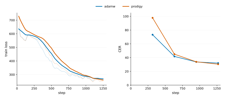
We try Prodigy in a small ASR (automatic speech recognition) experiment. We train on LibriSpeech [8] with both AdamW and Prodigy. This task was chosen because the original paper did not have audio experiments, but also because it is relatively cheap (code is here).

Specifically we trained a 6-layer Conformer [9] for 1 epoch on 100 hours of LibriSpeech using a character-level CTC loss. Note: this is very short compared to the original recipe, which trains on ~10x more data and for 500x more epochs on a 3x bigger model.

See Figure 1 for a comparison of the two optimizers. We did a coarse learning rate sweep for AdamW, and show the best AdamW run only. We used the default Prodigy settings. Final performance between AdamW and Prodigy is similar.

Interestingly, Prodigy takes a while to warm up. This is presumably due to $d_0$ being small at initialization; possibly increasing $d_0$ helps.

References

[1] Konstantin Mishchenko and Aaron Defazio (2024). Prodigy: An Expeditiously Adaptive Parameter-Free Learner, in Proceedings of the 41st International Conference on Machine Learning (ICML).

[2] Aaron Defazio and Konstantin Mishchenko (2023). Learning-Rate-Free Learning by D-Adaptation, in Proceedings of the 40th International Conference on Machine Learning (ICML).

[3] Maor Ivgi, Oliver Hinder, and Yair Carmon (2023). DoG is SGD’s Best Friend: A Parameter-Free Dynamic Step Size Schedule, in Proceedings of the 40th International Conference on Machine Learning (ICML).

[4] Francesco Orabona and Tatiana Tommasi (2017). Training Deep Networks without Learning Rates Through Coin Betting, in 31st Conference on Neural Information Processing Systems (NeurIPS).

[5] Greg Yang, Edward Hu, Igor Babuschkin, Szymon Sidor, Xiaodong Liu, David Farhi, Nick Ryder, Jakub Pachocki, Weizhu Chen, and Jianfeng Gao (2021). Tuning Large Neural Networks via Zero-Shot Hyperparameter Transfer, in 35th Conference on Neural Information Processing Systems (NeurIPS).

[6] Ashok Cutkosky, Aaron Defazio and Harsh Mehta (2023). Mechanic: A Learning Rate Tuner, in 37th Conference on Neural Information Processing Systems (NeurIPS).

[7] John Duchi, Elad Hazan, and Yoram Singer (2011). Adaptive Subgradient Methods for Online Learning and Stochastic Optimization, in JMLR.

[8] Vassil Panayotov, Guoguo Chen, Daniel Povey and Sanjeev Khudanpur (2015). Librispeech: An ASR corpus based on public domain audio books, in IEEE International Conference on Acoustics, Speech and Signal Processing (ICASSP).

[9] Anmol Gulati et al. (2020). Conformer: Convolution-augmented Transformer for Speech Recognition, in Interspeech (ISCA).

Appendix

A1, Design choices of Prodigy EMAs

The choices about which EMA quantities to track are somewhat arbitrary. The following choice is still sensible, $$ \begin{aligned} m_k' = d_k\mathrm{ema}(g)\quad v_k' = \mathrm{ema}(d^2g^2) \end{aligned} $$ since $$ \begin{aligned} -\frac{m_k'}{\sqrt{v_k'} + d_k\epsilon} \end{aligned} $$ still approaches the Adam direction if $d_k$ converges to a positive constant. However, one reason that $m_k = \mathrm{ema}(dg)$ could be preferable is that it down-weights steps where the $D$ estimate is bad.